Where this picks up
In our earlier case study, From MuJoCo to Real Hardware: Running RL Policies Through ROS 2, we described how Ekumen took a customer’s MuJoCo-trained policy for a robot manipulator and built the ROS 2 system around it. This post goes the other way. It takes you inside the learning loop, using the low cost, open-source Andino differential-drive platform.
A note on framing, up front: none of this is groundbreaking. We hope it is useful as an all-in-one reference with the concrete details to implement the controller.
The robot and the task
Andino is a fully open-source, ROS 2-native differential-drive robot: a Raspberry Pi, a 360° RPLIDAR A1M8, wheel encoders, all driven through ros2_control. It’s representative of a whole class of hobby- and education-grade mobile robots.
The task we set: follow a planned path across a small room and dock at the goal pose with sub-decimetre precision, while avoiding obstacles. In ROS 2 terms, we’re replacing the controller, that normally would be DWB (Dynamic Window Approach), with a learned policy.
One note on vocabulary: when we say “dock” we mean “park”, stop precisely at a target position and heading.
That last point matters and shapes everything below: the policy is a drop-in Nav2 nav2_core::Controller. It consumes a global plan and a costmap and emits velocity commands.
1. Setting up the learning loop
To train against MuJoCo with PyTorch, we wrap the physics in a standard Gymnasium environment. Stable-Baselines3 (SB3) drives the loop; the environment is the bridge between SB3’s tensors and MuJoCo’s physics state.
Each control step does four things:
- Observe. The environment reads MuJoCo’s state (chassis pose, velocities), projects the robot onto the planned path, and assembles an observation vector (details in §3).
- Infer. SB3 passes the observation through the policy network, which outputs a continuous, normalized action .
- Step. The environment maps that action to wheel velocities via differential-drive kinematics and steps MuJoCo
frame_skiptimes. - Reward. It computes a scalar reward and the next observation, and returns the transition to SB3.
MuJoCo’s physics runs at a 1 ms timestep, and we step it frame_skip = 33 times per control step. That’s ~30 Hz, matching the rate the controller runs on the real robot. Set the simulator’s control rate to the robot’s control loop, so the policy observes and acts on the same per-step dynamics in training and on hardware.
The action space is 2-dimensional and normalized to , mapped to physical limits:
Those bounds mirror the real Andino’s Nav2-DWB envelope (MAX_LINEAR_VEL = 0.2, MAX_ANGULAR_VEL = 1.0). That ratio between max linear and angular speed turns out to matter later, when we look at how the robot chooses to turn.
2. Choosing the learning method: SAC
For continuous control the two obvious candidates are SAC (Soft Actor-Critic) and PPO (Proximal Policy Optimization). We chose SAC.
Our SAC config: learning rate 3e-4, replay buffer 300k, batch 256, gamma = 0.999, automatic entropy tuning, 16 parallel environments, target 30M timesteps. The high discount factor is deliberate, at 30 Hz the long 5.5 m paths are hundreds of steps, and gamma = 0.999 is what lets the terminal docking bonus actually propagate back to the start of the episode. (At a lower 0.997 it was discounted to nothing over a long path, and the policy drove well but never bothered to nail the final pose.)
3. Small and geometric observation design
For obstacle awareness, the tempting default is a local costmap image fed through a CNN and fused with the physical state vector. However, we wanted a solid baseline before taking on that extra complexity.
We went small and geometric. The observation is a flat 24-dimensional vector, and the policy is a plain SB3 MlpPolicy with a [512, 512] architecture. The 24 dimensions break down as 16 state features + 8 obstacle “clearance probes”:
| Observation: flat Box(24,) | Notes | Size |
|---|---|---|
| v_fwd, ω | normalized velocities | 2 |
| 3 lookahead waypoints (x,y) | body-frame @ 0.2/0.4/0.8 | 6 |
| Path-heading error | scaled by 1/π | 1 |
| signed cross-track error | clipped to [-1,1] | 1 |
| dist-to-goal | Normalized /5 m | 1 |
| dist-in-goal-zone | Normalized /1 m (docking) | 1 |
| goal-heading error | As sin, cos | 2 |
| last action | 2 | |
| clearance probes | 8 fixed body-frame points costmap samples | 8 |
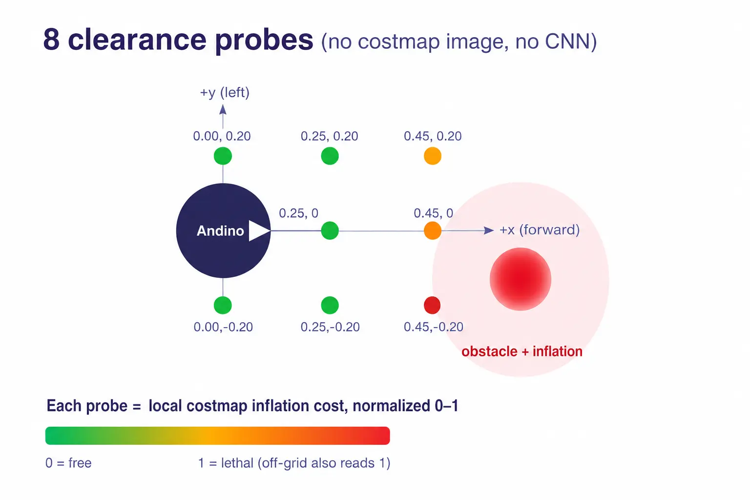
Instead of handing the policy a whole costmap picture and asking a CNN, we sample the costmap’s cost at 8 fixed points in the robot’s body frame (front, front-far, and the four diagonals), each normalized to (0 = free, 1 = lethal). This option is faster to train, and simpler to run on our target hardware (Raspberry Pi).
A handful of well-chosen, hand-placed features can get you most of the way. That said, the probes do trade away some information a costmap image would keep, mainly coverage, and any obstacle shape/motion cues a CNN could pick up on. If we push this further, the costmap-CNN approach is the natural next experiment.
4. The reward function
The agent’s normalized actions map to the physical limits from §1, and we shape behavior with a dense, multi-component reward. Roughly:
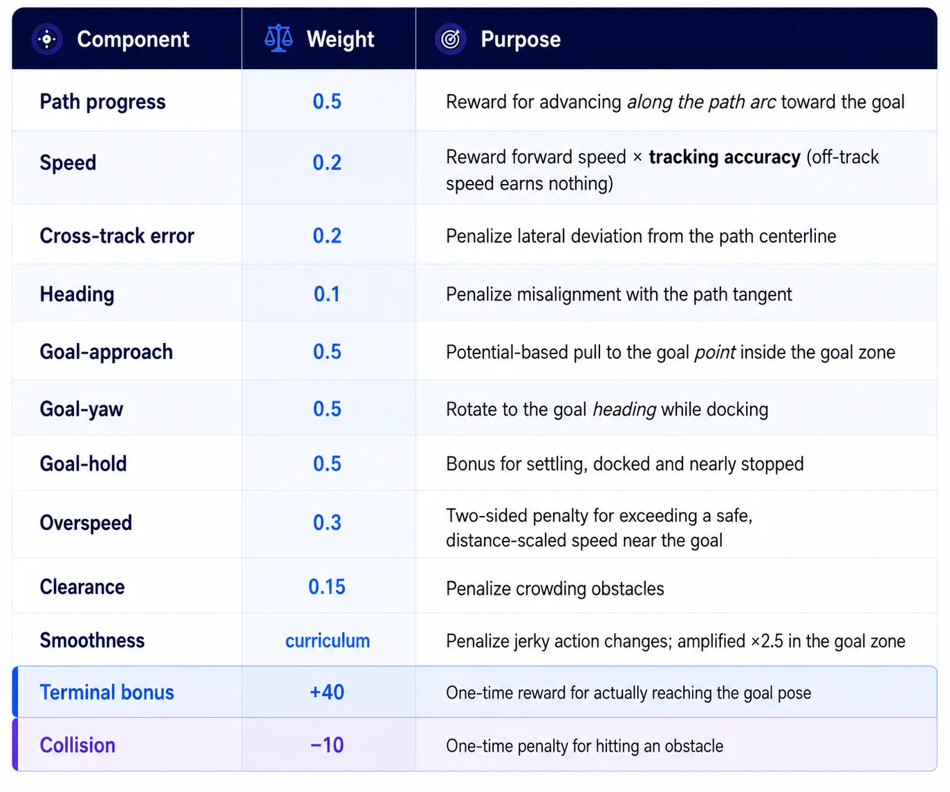
Two ideas do most of the work here:
Goal-zone blending. Within 1 m of the goal, the path-following terms fade out and the docking suite (approach, yaw, hold, overspeed) fades in. Path-arc progress saturates at the goal. The docking terms give it a smooth attractor at the exact goal pose and make overshooting or reversing explicitly negative. Splitting “drive” and “dock” into two regimes was key to produce clean stops.
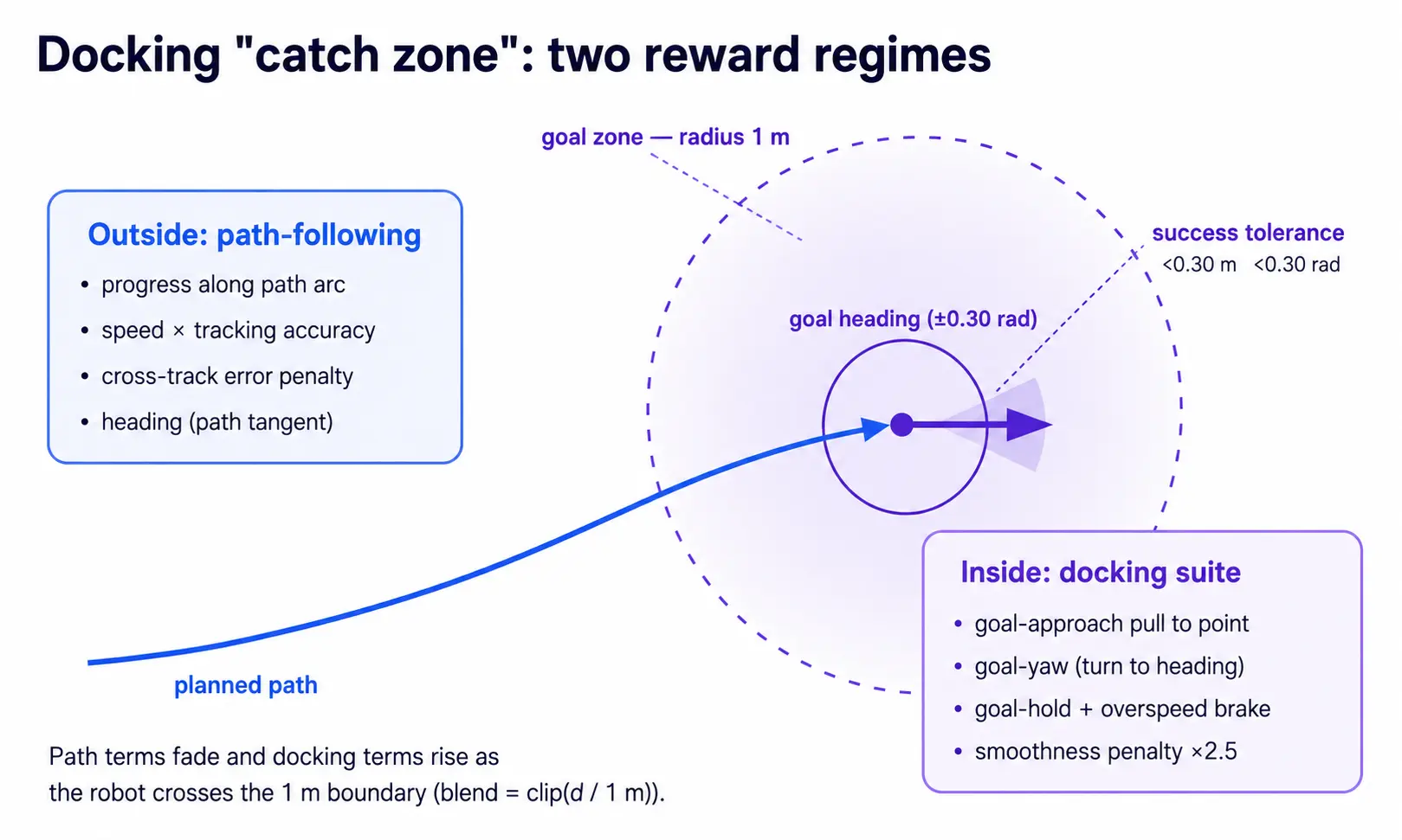
The terminal bonus has to be big. A full path traverse integrates the progress reward to hundreds. An early +10 terminal bonus was around 3% of the return and, discounted over a long path, effectively invisible. The policy learned to drive but not bother finishing. Raising it to +40, and adding the local, discount-friendly goal-zone terms, is what made completion compete with driving. Journey before destination, but we want to get there :) Check the terminal reward’s size against the shaping reward it has to compete with.
5. The curriculum
Learning to dock with decimetre precision at the end of a 5.5 m obstacle course, from scratch, is a sparse-reward problem that SAC will not solve if you just drop it in. We use an 8-level adaptive curriculum. Every level trains the same full task; only the difficulty ramps:
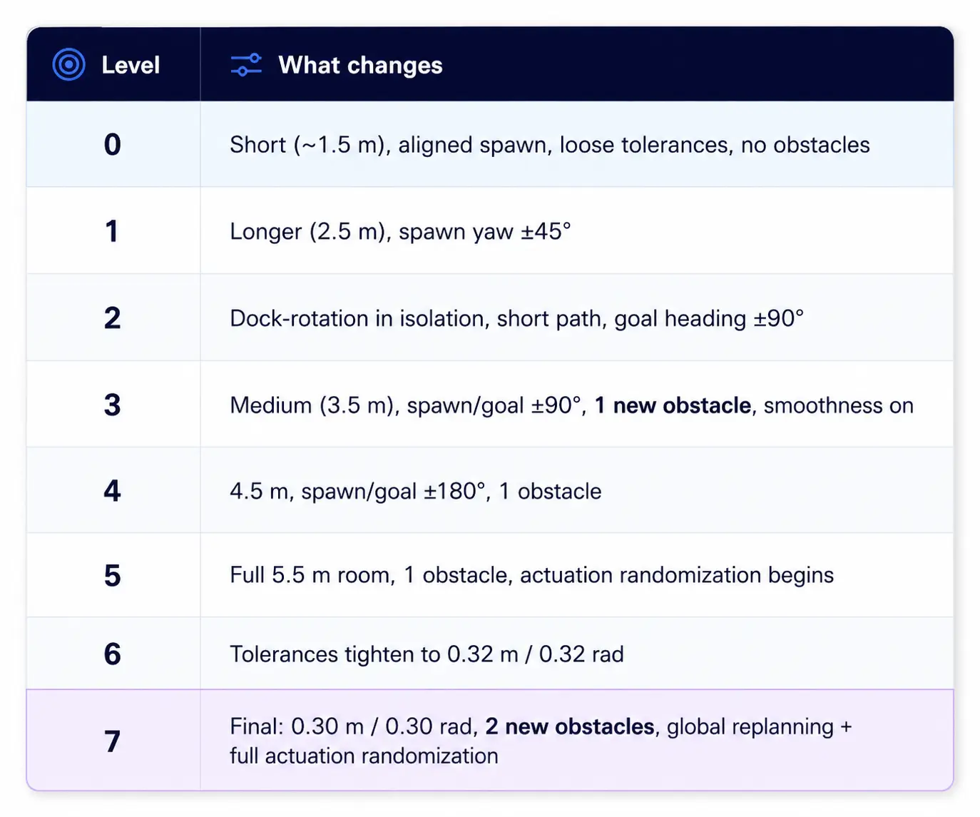
Progression is adaptive: promote when the rolling success rate (over 100 episodes) clears 0.6, demote if it falls below 0.25, with a grace period to stop the agent thrashing between two levels. The last two levels are where we “robustify”: we refresh the global plan under the robot (mimicking Nav2’s periodic replanning) and randomizing the actuation (rate limits, latency, scale, noise) to stand in for the unmodeled velocity smoother on the real robot. The policy learns clean tracking and docking first, then learns to be robust to the world shifting under it.
A practical note: the curriculum schedule lives in the config, not the code, so tuning it doesn’t mean touching the environment.
6. Verifying training success
We looked at training health along two axes: TensorBoard diagnostics during training, and a head-to-head benchmark against DWB before deployment.
TensorBoard: the failure modes to recognize
Most of debugging RL is learning to read the failure signatures. The four we hit repeatedly:
- Instant-failure loop. Success flat at 0, episodes extremely short. The robot drives off-track immediately. Usually too much initialization noise or too tight a starting corridor. Fix: ease the starting level.
- Reward hacking. Episode reward rises while success and progress stay at 0. For example, the agent farmed speed and heading rewards while ignoring cross-track error. This is insidious because the reward curve looks healthy. Fix: gate the rewards so they can’t be collected while misbehaving. For example: we multiply progress and speed by a forward-alignment gate and scale speed by .
- Mid-curriculum stall. Success plateaus below the promotion threshold at a specific level. Usually that level’s difficulty jump is too large; smooth the ramp.
- Catastrophic forgetting. Reward and success crash late in training after a destabilizing gradient update. Fix: lower the learning rate or raise the batch size.
Reward hacking is worth dwelling on, because it kept coming back in new forms. Every new reward term we added opened a new exploit. The docking suite fixed the “drives but won’t stop” problem and immediately introduced a fidgeting-in-place behavior, which we then had to fix with the goal-zone smoothness multiplier. Dense reward shaping is worth budgeting time for it. Next time, we’d invest earlier in a few adversarial “reward probes”—scripted policies that try to farm each term without doing the task—to catch these before long training runs.
Benchmark: RL vs DWB
Before deployment we run the evaluation suite, which drives 16 scenarios under both our RL policy and ROS 2’s default DWB controller, recording /odom, /cmd_vel_nav, and /scan. It reports:
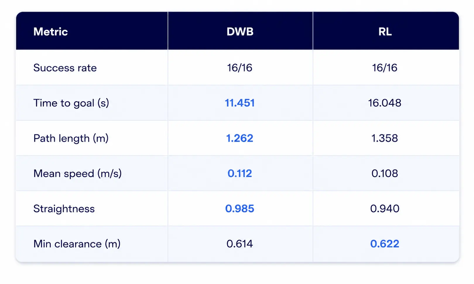
The RL policy is as reliable as DWB, and it gets there more slowly, over a slightly longer, less straight path. The pipeline produced a real nav2_core::Controller that drives the full task next to DWB!
The slower, longer-path part looked a problem at first. So we went looking for where the extra time and distance were going, expecting to find hesitation or wandering. We were surprised: it wasn’t a defect at all! (details in the next section).
So we’re happy with the controller: it’s as reliable as DWB, moved to hardware cleanly. The benchmark itself is what needs work (more runs, and metrics that credit the behaviour we want).
What worked
So where does that extra time and distance go? The answer is the nicest surprise of the project. A typical differential-drive robot does the following sequence: rotate in place to align with the path, drive straight doing small corrections, rotate again to the final heading. The learned policy resulted in a smoother and less-robotic motion. For most of a path it arcs forward through turns, keeping its speed. When the heading correction is large enough to be worth it, it backs up a bit, and rotates in two arcs instead of rotating in place.
That distinction is worth the reward-tuning effort on its own. A classical controller can be told to prefer arcs over rotations, but it does not usually work. Here, nobody wrote down “how to rotate gracefully”. The policy arrived at it on its own, because it’s what the incentives rewarded.
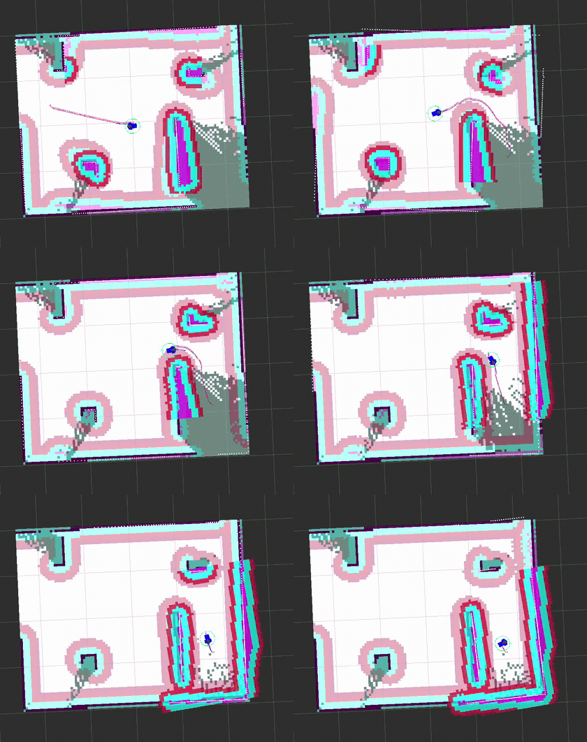
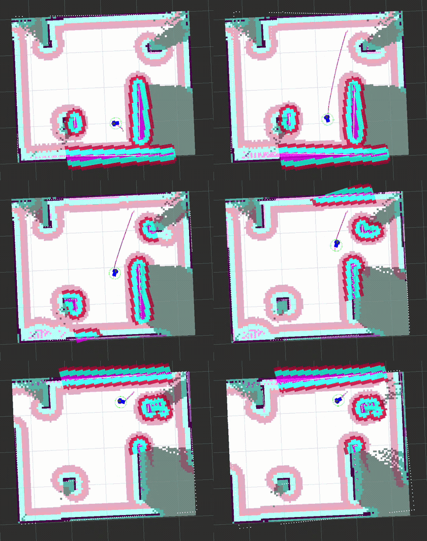
In hindsight, the incentives point right at it. The low angular-velocity ceiling (1.0 rad/s) relative to the linear speed (0.2 m/s) makes rotating in place slow, and the smoothness penalty punishes the sharp accel/brake of stopping and starting. For a small heading error, arcing through the turn while still making progress is cheaper than stopping to fix it. But the forward-alignment gating that rewards progress only while roughly facing the right way cuts the other direction for a large error: trying to arc through a near-reversal means pointing away from the goal for a long stretch, earning nothing, so doing an expensive correction first and then setting off is the better trade. The takeaway: you shape behavior through constraints and incentives, not by scripting the motion. You describe what good looks like in each situation, and the policy works out which response fits.
It’s also why the benchmark table above and this section don’t contradict each other. Those metrics reward straight-line efficiency; this behaviour spends a little of that efficiency to drive more naturally. What they don’t measure is how naturally a path was driven, and that’s squarely where the payoff shows up.
The other thing that worked: the policy navigated on the real Andino on the first attempt. No fine-tuning on hardware, no iterating against the real robot. We credit two things for that. First, a simulator that matches the deployment conditions closely (matching the control rate, the velocity envelope). Second, the actuation domain randomization introduced late in the curriculum, training against randomized rate limits, latency, scale, and noise meant the policy had already seen a range of “not quite what the sim predicted” dynamics during training.
The costs
- Training time. Reaching a deployable policy took roughly 9 hours on an RTX 5080 to hit ~30M timesteps across 16 parallel environments. That is not an afternoon, and every reward-shaping mistake or curriculum misstep costs you another multi-hour cycle. Sample efficiency (SAC) and parallel envs help, but the iteration loop is the real cost of RL here.
- Reward hacking, repeatedly. As covered in, every shaping term is an attack surface. Most of our calendar time went to this, not to the “learning.”
- Deploy parity is not free. The C++ controller needs to produce the same observations as the training code. Make sure to match configuration (inflation radius for example) between runtime and training.
We propose that training time is a substituted cost rather than extra cost. We’ve spent countless hours hand-tuning classical controllers to drive a robot well, and that work is slow and fragile. Hand-tuned parameters are bound to one robot in one regime. A training pipeline isn’t. Change the hardware, re-run training against the new dynamics (or fold that variation into domain randomization), and the policy works out the new “how” on its own. Weighed against the open-ended grind of manual tuning, a 9-hour training run is a good trade. The time you put into the training setup compounds; the time you put into hand-tuning gets spent again every time the robot changes.
Using the new controller
The trained policy exports to TorchScript (policy.pt plus a policy_metadata.json sidecar recording the observation/action layout, probe coordinates, lookaheads, and velocity limits). The export strips SB3’s stochastic sampling down to a deterministic tanh(μ) forward pass, with a determinism check that refuses to export if the traced model diverges from SB3’s own predict().
On the robot, that .pt is loaded by a C++ Nav2 controller plugin (LibTorch, CPU) that registers as a FollowPath controller — the same package runs unchanged in simulation and on the real Raspberry Pi.
Where this goes next
The thing we’re really handing over isn’t this particular policy — it’s the workflow that produced it: a sim matched to the robot’s control loop and velocity envelope, an observation defined by geometry so sim-to-real parity is a specification, and a curriculum that builds up to the full task.
Two threads we’d pull on from here:
- Richer obstacle awareness. The costmap-CNN is the natural next experiment.
- A benchmark worth trusting. More scenarios, better metrics, and a reproducible harness to run it all: Lambkin, Ekumen’s open-source benchmarking toolkit.
None of that changes the headline: a learned controller that drives more naturally than the classical baseline, trained in sim and deployed to real hardware on the first try.
Working on RL policy execution, ROS 2 navigation, or simulation-to-hardware integration? Talk to our robotics software team.