Building decent 3D maps takes time, effort, and resources. Portable LiDARs achieve great results, if you have one in your toolbox. 3D SLAM with AMRs is an option too, with careful calibration and tuning. So when we set ourselves to 3D map Ekumen HQ, and had neither at hand, we wondered. Can we do this with less? Can we do this with just a smartphone and open-source software — no expensive hardware, no complex rigs? That curiosity led us to experiment with different approaches to 3D reconstruction using an iPhone Pro. In this post, we share our process, the tools we used, and the lessons we learned while testing methods like NeRF, Gaussian Splatting, and others.
Why an iPhone Pro?
The iPhone Pro includes key sensors—such as LiDAR—and apps like NerfCapture or Stray Scanner App (using ARkit), which let you generate datasets with:
-
RGB images at 1920x1440 resolution
-
Depth maps at 256x192 resolution (LiDAR has a range of <5m)
-
Camera poses for each frame
-
The camera’s intrinsic matrix (without distortion model)
At some point, we also explored Android alternatives, since ARCore exposes similar data. However, depth images on Android are estimated by taking multiple device images from different angles and comparing them as a user moves their phone, and no recent phones with real depth sensors have been released (list of ARCORE devices). Source
What techniques were explored?
3D scene reconstruction from sparse posed images is commonly achieved by using intermediate 3D representations like neural fields, voxel grids, or 3D Gaussians. These approaches ensure multi-view consistency in both scene appearance and geometry.
With the goal of getting the best possible results — How NeRFs and 3D Gaussian Splatting are Reshaping SLAM: a Survey — and considering that we didn’t need real-time processing and with an NVidia RTX 4090 at hand, we decided to test InstantNGP and SplaTAM.
Let’s break down the main options we explored:
Neural Radiance Fields (NeRFs)
NeRFs are represented as a continuous 5D function that outputs the radiance emitted in each direction (θ, φ) at each point (x, y, z) in space, and a density at each point which acts like a differential opacity cotrolling how much radiance is accumulated by a ray passing through (x, y, z). A multilayer perceptron (MPL) neural network can be trained to represent this function by regressing from a single 5D coordinate (x, y, z, θ, φ) to a single volumen density and view-dependent RGB color. Source
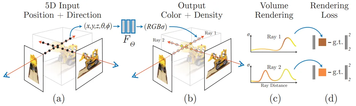
The figure below shows a basic overview of NeRF’s process: sampling along camera rays, feeding points to a neural network, and using volume rendering to produce an image. Optimization is done by minimizing the difference between synthesized and real images.
 |
|---|
| An overview of our neural radiance field scene representation and differ-entiable rendering procedure. The algorithm renders images by (a) sampling 5D coordinates (location and viewing direction) along camera rays, (b) feeding those locations into an MLP to produce a color and volume density, and (c) using volume rendering techniques to composite these values into an image. This rendering function is differentiable, so (d) we can optimize our scene representation by minimizing the residual between synthesized and ground truth observed images. Source |
Gaussian Splatting
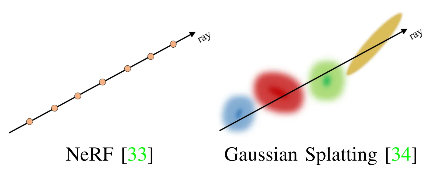
Gaussian Splatting is a method that uses an explicit 3D point cloud of “gaussian splats”—each one defined by position, size, color, and shape. It’s much faster to train and render compared to NeRFs, and it has become popular thanks to its balance between speed and quality. Below is a conceptual comparison between NeRF and 3DGS methods:
 |
|---|
| NeRF and 3DGS differ conceptually. (left) NeRF queries an neural network along the ray, while (right) 3DGS blends Gaussians for the given ray. source |
As alternative methods, we also considered COLMAP, a Structure-from-Motion (SfM) and Multi-View Stereo (MVS) tool that relies on geometry and feature matching between images to reconstruct the 3D scene; and different SLAM techniques widely used in robotics, which are typically much faster but usually produce lower-quality maps.
Experiments
NeRF Capture + InstantNGP
NeRF Capture offers two modes: Online mode and Offline mode. We went for Offline mode to avoid walking around with a desktop computer on our backs.
After recording, NeRF Capture provides a script to convert the dataset into the NeRF format for InstantNGP. Setting the aabb_scale parameter correctly in transforms.json was important to properly focus the scene.
Our first results looked promising visually, but using Instant-NGP mesh generator to create an OBJ from the NeRF didn’t yield the quality we were looking for. Below, we show a visual comparison between the NeRF and the extracted mesh.


SplaTAM + NeRF Capture
In order to load the datasets recorded with NeRF Capture, SplaTAM provides the nerfcapture2dataset.py script, which processes the dataset so it matches the expected directory structure for SplaTAM. Some of the work involved modifying the script to work with Offline mode, allowing us to load a previously recorded dataset instead of working with Online mode.
After running the SplaTAM algorithm, the output was saved into a params.npz file format, which could then be visualized with Open3D Viewer to get a hold of the generated point cloud.
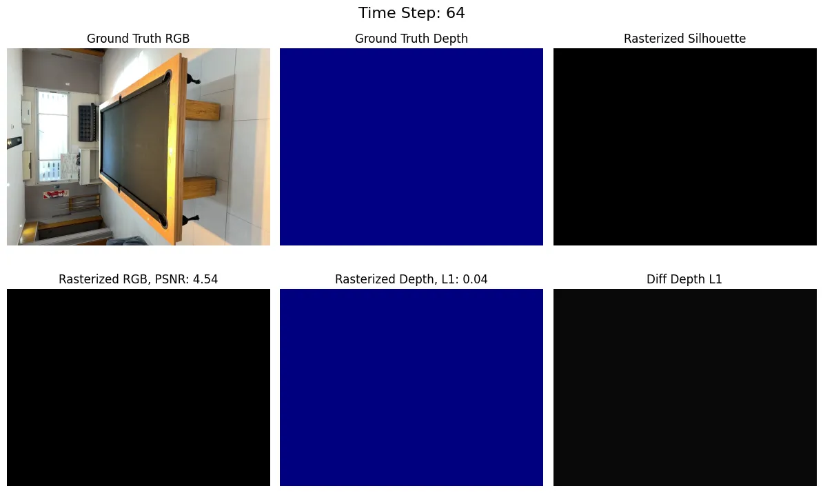
Alongside this, a metrics plot showing the PSNR and the captured depth for each frame was generated, and additionally, each output frame was rasterized.
This approach, although it got us as far as running the SplaTAM algorithm, didn’t give us the 3D map we were looking for. The results showed no information about the surrounding depth. After a while, we realized that the datasets were not saving the depth data correctly, as NeRF Capture author states in this comment; therefore, there essentially was no depth information for SplaTAM to work with. So we had to move on from using NeRF Capture Offline mode.
Splatam + Spectacular AI
The process here was mostly the same as with NeRF Capture + SplaTAM, except that we completely replaced NeRF Capture recording with Spectacular AI. The key difference here was that Spectacular AI correctly saved the depth data, which helped us get some useful results from SplaTAM.
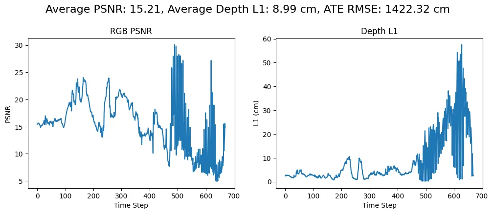
Although results started to look better, we still had to discard some parts of the recordings in order to get some useful data to work with. For example, the plot below to the right shows the recorded depth while recording around a 10 square meters room.
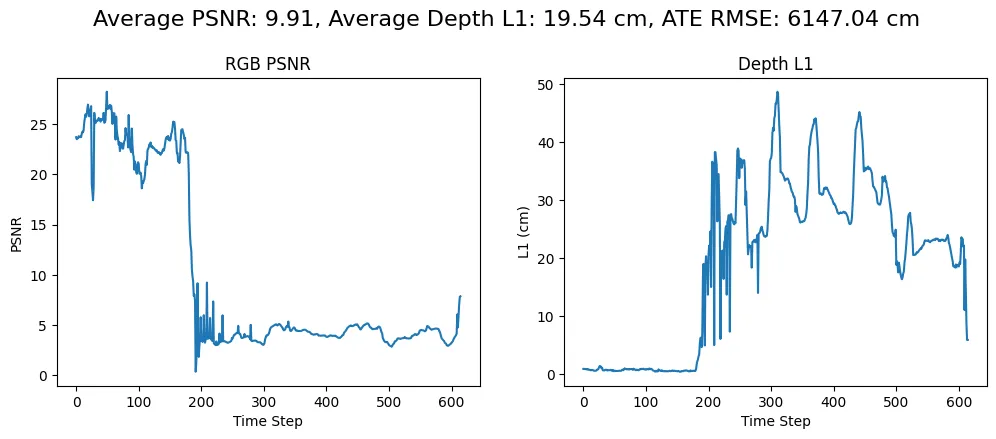
After visualizing the results from the dataset related to that plot, it became clear that the device tracking had some issues when processing.
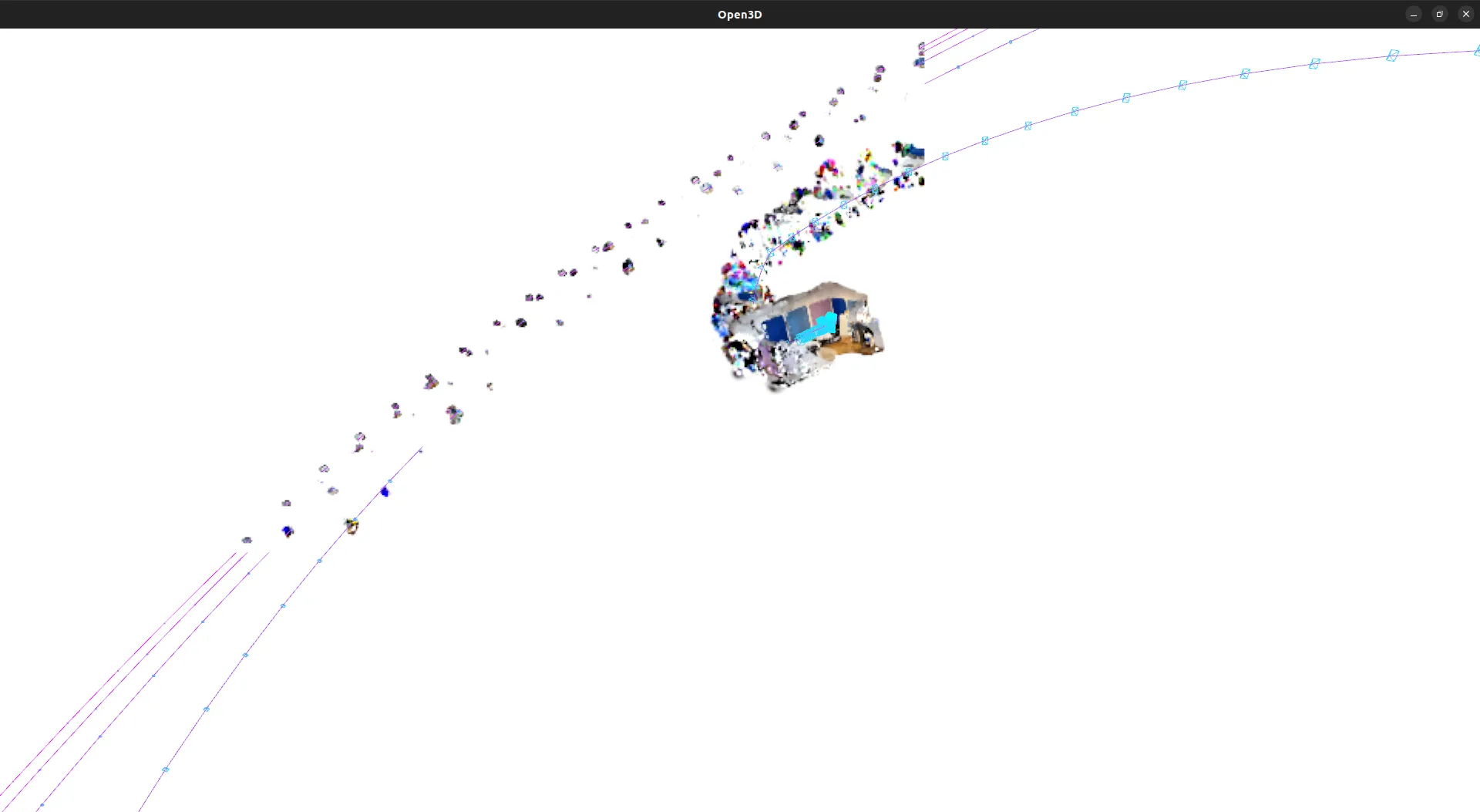
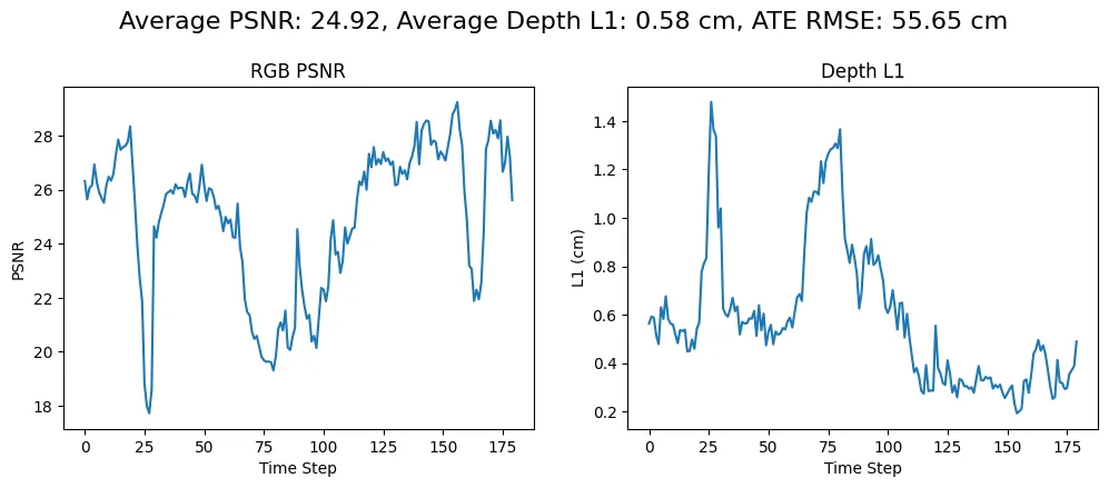
Running SplaTAM again, keeping the frames up to the depth graph first peaks (around 180 time steps), removed all the malformed data, and gave us results like the ones below. Still not ideal to map 3D closed spaces, but starting to show some interesting results.

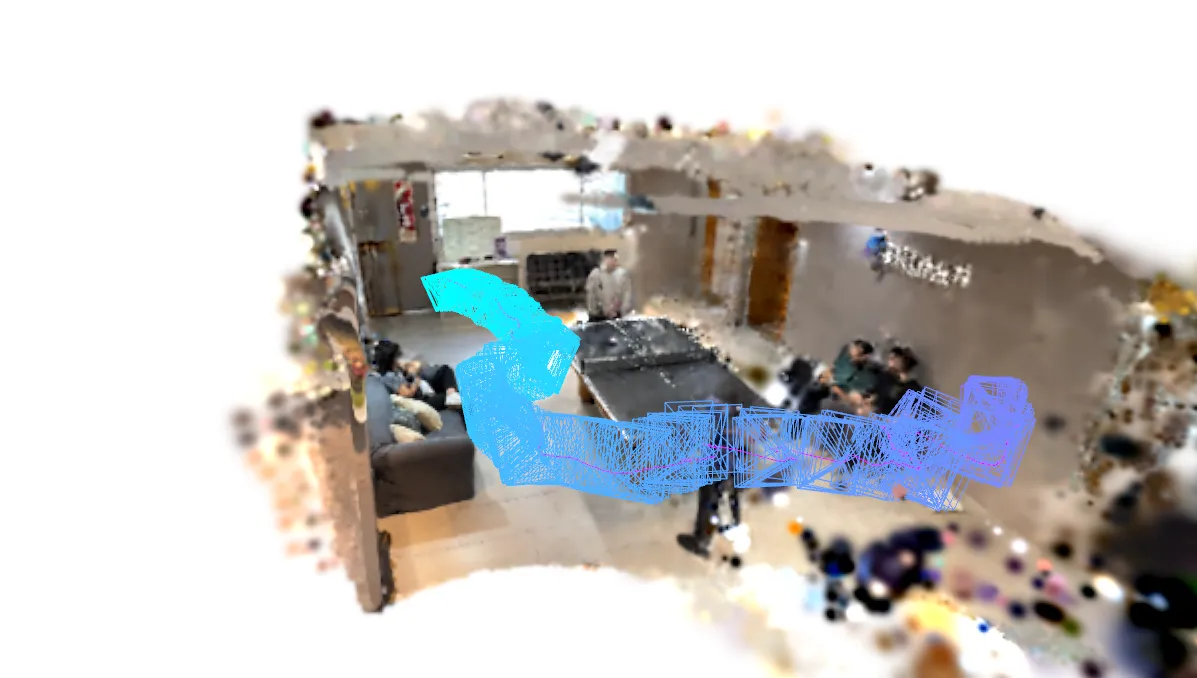
The same procedure was followed to map the surroundings of another room with some people in it.
Conclusion
Our experiments showed that creating detailed 3D maps with just a smartphone and open-source tools is definitely possible, but with limitations. Clean depth data is critical. NeRFs can deliver amazing visual quality at the cost of heavy processing, while Gaussian Splatting offers a much faster path to usable maps.
While we couldn’t achieve a perfect reconstruction yet, the exploration helped us understand the strengths and weaknesses of each method—and where data quality becomes a bottleneck.
What’s next: In our next post, we’ll take a closer look at the data itself—using the Stray Scanner App combined with Open3D to better understand, visualize, and prepare datasets for future reconstructions. Stay tuned as we dig deeper into the math behind the scenes!