Modeling LeKiwi’s omni-base in MuJoCo

A bit of context…

If you are involved in robotics and communities like HuggingFace, you have probably heard about LeKiwi already. LeKiwi is a low-cost, open-source, and 3D-printable mobile manipulator robot. It is primarily designed for research, education, and prototyping in the fields of robotics and embodied AI. The robot can be used via LeRobot software, and its use is straightforward; however, to speed up development, we encountered the need for a simulation that could serve as a drop-in replacement for the real robot. At Ekumen, we use it as a guinea pig for some research prototypes and for internal training. You can test it yourself at Ekumen-OS/lekiwi.

The Magic of Omni-Wheels

Simulation always implies approximation; even when having complex mathematical models, you are at some point simplifying reality and committing to an error that is within your tolerance. Nonetheless, the first step is always the same: “Let’s understand the real case.”

The Omni-Wheel principle

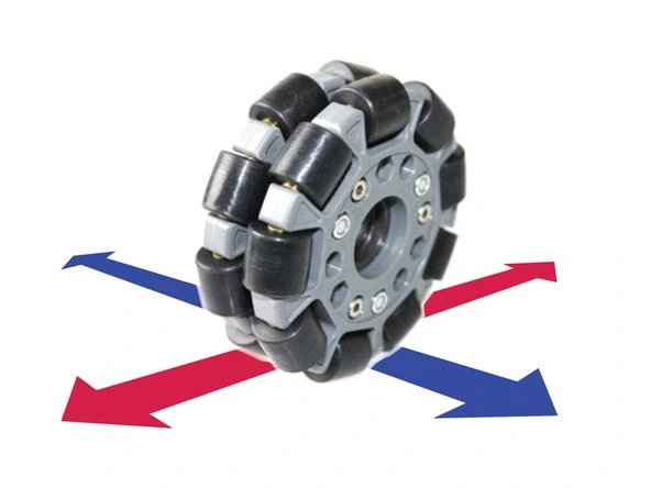
An omni-wheel is a standard-looking wheel with one major difference: its circumference is lined with small rollers (typically perpendicular to the wheel’s main axle).

In the driving direction (forward/backward), the wheel grips and behaves like a normal wheel.
In the lateral direction (sideways), the rollers spin freely, allowing the wheel to slide with very low friction.

This combination of grip in one direction and slip in another, plus a correct setup of the wheels to allow control in all directions, is what enables holonomic movement—the ability to move in any direction, regardless of the robot’s orientation.

Difference: Omni-Wheels vs. Mecanum Wheels

People often confuse omni-wheels with mecanum wheels. The difference is subtle but crucial:

Omni-Wheels: Rollers are perpendicular to the wheel’s axis of rotation (or parallel to the axle).
Mecanum Wheels: Rollers are mounted at a 45-degree angle to the wheel’s axis.

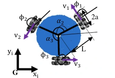
This 45-degree offset on mecanum wheels means a 4-wheel configuration can cleverly balance forces to strafe (move sideways) directly. Omni-wheel systems achieve this through their arrangement, most commonly a 3-wheel setup, where the wheels are distributed around the periphery of a circumference at 120-degree intervals.

Kinematic Principle of Lekiwi’s Base

Lekiwi utilizes a 3-wheeled omni-base, with the wheels typically arranged 120 degrees apart. While this configuration is a classic solution for holonomic movement, understanding why it works requires looking at the underlying wheel mechanics before applying simple vector math.

The key lies in the physical construction of the omni-wheels. As mentioned previously, these wheels feature passive rollers along their circumference that rotate perpendicular to the wheel’s drive direction. This mechanical feature effectively creates force decoupling:

When one wheel drives forward, it relies on longitudinal friction to push the robot.
Simultaneously, the rollers on the other wheels spin freely, minimizing transverse friction and preventing “drag.”

Because the passive rollers negate resistance in the non-drive directions, the motion of each wheel is kinematically decoupled from the others. This allows us to model the robot’s total velocity as a linear combination of the three individual wheel speeds. By superimposing the velocity contributions of the three wheels, we can precisely control the resultant speed and direction to achieve true holonomic motion.

We are not going to dive into the kinematic solution as it is not the goal of this post, but it is important to understand the expected behavior to correctly model it. For further information on the kinematics, you can have some fun during the weekend by applying some trigonometry, or you can check references like:

Modeling Omni-Wheels in MuJoCo

As built-in omniwheel object is not provided by MuJoCo, this behavior must typically be constructed from its fundamental physics primitives.

There are at least three different paths that can be followed to model this type of wheel in MuJoCo:

Model the rollers (The “High-Fidelity” route):
- Model the main wheels and each individual perpendicular roller as a separate geom with its own joint.
- Using cylinders as primitives, you can model both the main wheel and the rollers.
- This is the most structurally accurate; you are relying entirely on the physics engine to calculate the forces that make the wheels move in the expected directions. The downside of this is the computational cost, as more dynamic joints are used in the model, and the simulation stability due to the comparatively higher number of contact forces acting on each complex wheel.
Model frictions (The “Compromised and yet Smart” route):
- Model the wheel as a single simple shape (cylinder/capsule/sphere). Then, use MuJoCo’s friction properties to imitate the omni-wheel’s behavior: high friction in the rolling direction(we want the wheel to spin), and low friction in the lateral direction, as if the rollers were there.
- This is computationally fast, and it is an elegant way to skip the “High-Fidelity” route by relying on friction modelization. On simple surfaces, the kinematics would match the real case scenario. While this method necessitates a comprehensive grasp of MuJoCo’s friction models, the additional contacts computed in Option 1 yield higher accuracy on complex surfaces, as long as we are able(and MuJoCo lets us) to tune the parameters correctly.
Simplify to regular wheels (The “Wrong” route):
- Model them as simple cylinders with standard friction. The base will move, but the friction for lateral sliding of the wheels opposing the movement of the base might cause a wrong velocity computation.
- Easiest solution, it might be useful during a confined-hours hackathon, but it completely defeats the purpose of the omniwheel if we want to do things right.

Even though we considered Option 1, we went for Option 2, not only because it was presented like the smart route, but also because it presents a good balance between fidelity and computation expense, a trade-off that you might have encountered before if working as simulation engineers.

MuJoCo’s isotropic vs anisotropic frictions

Traditional textbooks usually distinguish between static friction (holding an object in place) and dynamic friction (resisting motion while sliding), where typically $\mu_{\text{static}} > \mu_{\text{dynamic}}$ .

MuJoCo treats friction as a contact constraint rather than just a force. It solves for contact forces within a defined friction cone (and then relies on a pyramidal approximation for computational efficiency).

The simulator calculates (constraints solver) the force required to prevent motion. If this force is inside the friction cone, the object sticks (static behavior). If the force hits the limit of the cone, the object slides (dynamic behavior).

MuJoCo is highly tunable. While the default behavior assumes isotropic friction, the solver can be configured to handle complex anisotropic interactions. For the sake of simplicity and to avoid complicating things, we are focusing only on sliding friction using a contact dimension of 3 (See geom-condim), which already provides sufficient room for presenting this case. When using contact parameters, the model allows you to indicate the contact dimension for your friction cone: The higher the dimension, the more tunability you have for the friction.

Note: For a deep dive into the math behind soft contacts and convex optimization, referencing the Computation section of the MuJoCo documentation is highly recommended.

Isotropic friction

This is the standard Coulomb friction model taught in introductory physics and is the default behavior for most objects in MuJoCo.

Isotropic means “uniform in all directions”; an object with isotropic friction will create the same amount of force when sliding in any direction (forward, backward, diagonal).

When you define a <geom> you use the friction attribute with three values: friction="[sliding, torsional, rolling]". The first value is a single number. The said coefficient is applied to any sliding direction in the contact plane, making it isotropic.

<mujoco model="cube_isotropic">
  <asset>
    <texture name="grid" type="2d" builtin="checker" rgb1=".1 .2 .3" rgb2=".2 .3 .4" width="512" height="512"/>
    <material name="grid" texture="grid" texrepeat="1 1" texuniform="true" reflectance=".2"/>
  </asset>

  <worldbody>
    <light pos="0 0 1.5" dir="0 0 -1" directional="true"/>
    <geom name="floor" pos="0 0 0" size="5 5 .05" type="plane" material="grid"/>
    <body name="cube" pos="0 0 .3">
    <!-- I want to move it along x,y and z and rotate only around z. That's why I am not using a free joint type -->
      <joint type="slide" axis="1 0 0"/>
      <joint type="slide" axis="0 1 0"/>
      <joint type="slide" axis="0 0 1"/>
      <joint type="hinge" axis="0 0 1"/>
      <geom name="cube" type="box" size="0.1 0.1 0.1" friction="1.0 0.05 0.001"/>
    </body>
  </worldbody>
</mujoco>

The cube was defined with an isotropic sliding friction of 1., so when a force is applied in any direction of the contact frame, the contact forces are strong enough to quickly stop the cube from sliding. (See MuJoCo-contact)

Anisotropic friction

This is a more advanced, specialized model used to simulate objects that slide more easily in one direction than another.

When using anisotropic friction, the friction forces change depending on the direction of the slide. The perfect example is the ice skate.

Sliding forward/backward (along the blade) has very low friction
Sliding sideways (perpendicular to the blade) has very high friction

In MuJoCo, anisotropic friction is typically defined as a contact parameter, not on the <geom> tag itself. In other words, to define friction that is different in the X-axis versus the Y-axis, the physics engine needs to know exactly where those axes are pointing.

Anisotropic friction relies on the contact frame. A generic collision between two objects does not guarantee a consistent alignment of the contact tangent vectors. By defining a specific <pair>, you implicitly define a stable contact frame. The friction coefficients are then calculated with respect to this specific frame and the defined friction model.

The friction field in this case will give you the chance to define sliding friction for two directions in the contact frame: “friction="[fric_tangent_1, fric_tangent_2, fric_torsional, fric_rolling_1, fric_rolling_2]" (Note: the dimension will depend on the contact dimension being used)

<mujoco model="cube_isotropic">
  <asset>
    <texture name="grid" type="2d" builtin="checker" rgb1=".1 .2 .3" rgb2=".2 .3 .4" width="512" height="512"/>
    <material name="grid" texture="grid" texrepeat="1 1" texuniform="true" reflectance=".2"/>
  </asset>

  <worldbody>
    <light pos="0 0 1.5" dir="0 0 -1" directional="true"/>
    <geom name="floor" pos="0 0 0" size="5 5 .05" type="plane" material="grid"/>
    <body name="cube" pos="0 0 .3">
    <!-- I want to move it along x,y and z and rotate only around z. That's why I am not using a free joint type -->
      <joint type="slide" axis="1 0 0"/>
      <joint type="slide" axis="0 1 0"/>
      <joint type="slide" axis="0 0 1"/>
      <joint type="hinge" axis="0 0 1"/>
      <geom name="cube" type="box" size="0.1 0.1 0.1" friction="0.8 0.05 0.001"/>
    </body>
  </worldbody>

  <contact>
    <!-- Override default friction -->
    <pair name="non-isotropic" geom1="floor" geom2="cube" condim="3" friction="0 1"/>
  </contact>
</mujoco>

In this case, the cube presents an anisotropic sliding friction of [0, 1]. Meaning that in one tangent direction the friction is zero while in the other tangent direction is one. (We are going to talk about the reference frame shortly.) When the cube is moved along one direction of the contact frame, its null friction keeps the cube sliding indefinitely, while moving the cube in the other, perpendicular direction, it gets stopped almost immediately due to the large friction in that direction.

MuJoCo’s contact frame orientation

If you carefully watched the previous examples, you might have noticed that the contact frames of the contact points in the cube are always oriented in the same direction. So the “orientation” of the sliding friction tangent is always pointing to the same direction (in the world frame), no matter how the cube is actually oriented!

This is a known limitation: “Anisotropic friction is tightly coupled to the specific collider used, as the collider determines the orientation of the contact frame”(See #mujoco/issues/67) For instance, in the case of the cube, the contact frame is always oriented the same way in the world frame, no matter how the cube is rotated.

If you are thinking ahead, you might foresee that this could be a real complication for our omniwheel modeling. We need the contact frame to be oriented somehow relative to the omniwheel orientation. Otherwise, it wouldn’t be useful for our case.

Spoiler alert! For the cylinder, which is probably the most used geometry to model a wheel, it also has the same issue as the box orientation for the contact frame orientation. Luckily, for the capsule, the contact frame orientation changes along with the orientation of the capsule’s longitudinal axis.

Here a demo scenario where contact frames are tested for different geometries:

<mujoco model="ice skate">
  <asset>
    <texture name="grid" type="2d" builtin="checker" rgb1=".1 .2 .3" rgb2=".2 .3 .4" width="512" height="512"/>
    <material name="grid" texture="grid" texrepeat="1 1" texuniform="true" reflectance=".2"/>
  </asset>

  <worldbody>
    <light pos="0 0 1.5" dir="0 0 -1" directional="true"/>
    <geom name="floor" pos="0 0 0" size="5 5 .05" type="plane" material="grid"/>
    <body name="capsule_body" pos="0 0 .3">
    <!-- I want to move it along x,y and z and rotate only around z. That's
    why I am not using a free joint type -->
      <joint type="slide" axis="1 0 0"/>
      <joint type="slide" axis="0 1 0"/>
      <joint type="slide" axis="0 0 1"/>
      <joint type="hinge" axis="0 0 1"/>
      <geom type="box" size=".03 .02 .2"/>
      <geom name="end_capsule" type="capsule" fromto=".0 0 -.25 .1 0 -.25" size=".05"/>
    </body>
    <body name="cylinder_body" pos="-2 0 .3">
      <joint type="slide" axis="1 0 0"/>
      <joint type="slide" axis="0 1 0"/>
      <joint type="slide" axis="0 0 1"/>
      <joint type="hinge" axis="0 0 1"/>
      <geom type="box" size=".03 .02 .2"/>
      <geom name="end_cylinder" type="cylinder" fromto=".0 0 -.25 .1 0 -.25" size=".05"/>
    </body>
    <body name="sphere_body" pos="2 0 .3">
      <joint type="slide" axis="1 0 0"/>
      <joint type="slide" axis="0 1 0"/>
      <joint type="slide" axis="0 0 1"/>
      <joint type="hinge" axis="0 0 1"/>
      <geom type="box" size=".03 .02 .2"/>
      <geom name="end_sphere" type="sphere" size=".05" pos=".0 0 -.25"/>
    </body>
  </worldbody>

  <contact>
    <pair name="non-isotropic_1" geom1="floor" geom2="end_capsule" condim="3" friction="0.01 1"/>
    <pair name="non-isotropic_2" geom1="floor" geom2="end_cylinder" condim="3" friction="0.01 1"/>
    <pair name="non-isotropic_3" geom1="floor" geom2="end_sphere" condim="3" friction="0.01 1"/>
  </contact>
</mujoco>

In the video above, three different bodies are forced to move, each one of them has a different geometry type making contact with the ground: Cylinder, Sphere and Capsule. In the first and second cases, the same thing happens: the contact frames’ orientation is aligned with the world frame, though the object is being rotated. In the third case, when applying a force to the body with a capsule at the end, we can see that the orientation of the contact frame changes with the orientation of the geometry. This is the case of the ice skate that was mentioned earlier. When moving this in the longitudinal direction, almost no friction force opposes the movement, while when moving this laterally, the object stops almost immediately due to high friction in that direction.

What we need is to use capsule geometries to model the omniwheels for the LeKiwi.

Modeling the 3-omniwheel base

Now that we know how to set up the anisotropic friction and we analyzed the geometries to understand the contact frame, let’s do a quick proof-of-concept disposing the omniwheels in a 3-wheeled setup. As we mentioned before, as the contact frame depends on the collider being used, we are relying on the capsule geometry to model the omniwheels.

Note that below we are defining contact pairs between the floor and the wheels, and there we are defining the two friction tangent directions: low friction when sliding laterally, to simulate the effect of the rollers in the omniwheel, and high friction when sliding longitudinally, for the wheel to correctly spin forward and backward.

<mujoco model="omniwheel_base_demo">
    <compiler angle="radian" />
    <asset>
        <texture type="2d" name="groundplane" builtin="checker" mark="edge" rgb1="0.2 0.3 0.4" rgb2="0.1 0.2 0.3"
          markrgb="0.8 0.8 0.8" width="300" height="300"/>
        <material name="groundplane" texture="groundplane" texuniform="true" texrepeat="5 5" reflectance="0.2"/>
        <material name="black" rgba="0 0 0 1"/>
    </asset>

    <default>
        <default class="wheel_hub">
            <geom type="mesh" mesh="wheel_hub" pos="0 0 0" euler="0 0 0" />
            <joint type="hinge" axis="0.0 0.0 1.0" pos="0.0 0.0 0.0" />
        </default>
        <default class="omniwheel_collision">
            <geom type="capsule" size="0.051 0.01" pos="0 0 0" euler="0 0 0"
                  friction="0.8 0.05 0.001" group="0" />
        </default>
    </default>

    <actuator>
        <velocity name="base_left_wheel" joint="base_left_wheel_joint" kv="1" ctrlrange="-2. 2."/>
        <velocity name="base_right_wheel" joint="base_right_wheel_joint" kv="1" ctrlrange="-2. 2."/>
        <velocity name="base_back_wheel" joint="base_back_wheel_joint" kv="1"  ctrlrange="-2. 2."/>
    </actuator>

    <worldbody>
        <light pos="0 0 1.5" dir="0 0 -1" directional="true"/>
        <geom name="floor" pos="0 0 -0.1" size="0 0 0.05" type="plane" material="groundplane"/>
        <body name="base_plate_layer_1_link" pos="0.0 0.0 0.0" euler="0.0 0.0 0.0">
            <geom name="base_plate_layer_1_geom" type="cylinder" size="0.08 0.005" pos="0 0 0.06" rgba="0.4 0.01 0.4 1"/>
            <joint type="free"/>
            <body name="wheel_hub_back_link" pos="-0.1075 0. 0" euler="1.5708 1.5708 0">
                <joint name="base_back_wheel_joint" class="wheel_hub" />
                <geom name="wheel_back_geom" class="omniwheel_collision" material="black"/>
            </body>
            <body name="wheel_hub_left_link" pos="0.05375 0.0931 0" euler="1.5708 -0.5236 0">
                <joint name="base_left_wheel_joint" class="wheel_hub" />
                <geom name="wheel_left_geom" class="omniwheel_collision"/>
            </body>
            <body name="wheel_hub_right_link" pos="0.05375 -0.0931 0" euler="1.5708 0.5236 0">
                <joint name="base_right_wheel_joint" class="wheel_hub" />
                <geom name="wheel_right_geom" class="omniwheel_collision"/>
            </body>
        </body>
    </worldbody>

    <contact>
      <pair name="non-isotropic_1" geom1="floor" geom2="wheel_back_geom" condim="3" friction="0.01 1." solref="0.10 0.7" solimp="0.3 0.6 0.001"/>
      <pair name="non-isotropic_2" geom1="floor" geom2="wheel_left_geom" condim="3" friction="0.01 1." solref="0.10 0.7" solimp="0.3 0.6 0.001"/>
      <pair name="non-isotropic_3" geom1="floor" geom2="wheel_right_geom" condim="3" friction="0.01 1." solref="0.10 0.7" solimp="0.3 0.6 0.001"/>
    </contact>
</mujoco>

In the demo, we are using a particularly large size to better show the rotation of the wheels. Using the GUI’s joint controller and respecting the kinematics of the system, the base is moved forward/backward and to the sides to verify the correct behavior of our model.

LeKiwi’s base MuJoCo sim

This very same approach can then be applied to the complete LeKiwi model.

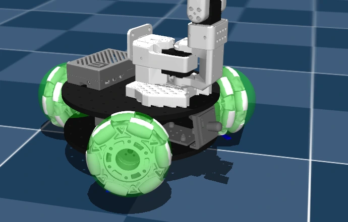
In the LeKiwi MuJoCo model, we defined two different types of <geom> for the wheels:

Mesh-based geom for the visuals
- Collisions are disabled.
Capsule geom for the collision calculations. (Painted in green in the image for references)
- Visuals are disabled.

The final MuJoCo model of the LeKiwi robot can be found at https://github.com/Ekumen-OS/lekiwi/../lekiwi.xml

Conclusions & Takeaways

Modeling omni-wheels in simulation is a classic physics problem that perfectly highlights the trade-offs between physical accuracy and computational cost. This guide demonstrates that a clever application of MuJoCo’s advanced features can achieve a high-fidelity, high-performance result without the computational nightmare of modeling every single roller.

Here are the key takeaways from the process of modeling the LeKiwi’s omni-base:

Choose the Right Modeling Path: While modeling every individual roller is the most physically accurate (“High-Fidelity”) route, it’s computationally expensive and complex. The “Smart” route—simulating the effect of the rollers using anisotropic friction—provides the best balance of realism and performance for most robotics applications.
Anisotropic Friction is the Key: Omni-wheels, by design, have different friction properties in different directions (high friction for rolling, low friction for lateral sliding). This cannot be modeled with standard isotropic friction. You must use MuJoCo’s anisotropic friction capabilities, typically defined in the <contact> section.
The Most Critical “Gotcha”: Geom Type Matters: For cylinder and box (and others) geometries, the anisotropic friction contact frame orientation is fixed relative to the world, not the object. This makes it useless for a rotating wheel.
- The capsule geometry is the workaround for this solution. Its contact frame rotates with the capsule’s longitudinal axis, which is exactly the behavior needed. By modeling the omni-wheels as capsules, you can ensure the low-friction direction (simulating the rollers) and high-friction direction (for rolling grip) are always correctly aligned with the wheel.