Introduction

Nav2 AMCL has two different implementations of the likelihood sensor model. In this post we look into how they compare to each other and what the performance implications are for your robot.

Improbable math

Something funny happened while we were evaluating the Nav2 AMCL node for the Beluga project: the two main sensor models in the Nav2 AMCL node, the likelihood_field and the beam, are both almost to-the-letter implementations of the namesake sensor models described in the well-known Probabilistic Robotics book by Thrun et al.

Almost, because if you look carefully to the likelihood field and beam model implementations, you’ll notice that Nav2 AMCL aggregates probabilities a bit different than the book.

The conventional way to work with a sensor scan like this is to make the weight of each particle equal to the probability or likelihood of the scan given the particle’s pose. This is calculated by multiplying the probabilities of each of the beams in the scan, assuming they are statistically independent.

Where $z$ is the measurement, $x_i$ is i-th particle’s state (pose), and $N$ is the number of beams in a scan. This is the way this is done in Thrun’s book.

However, both the likelihood_field and the beam models in Nav2 AMCL give this a twist. Their code actually implements this formula:

What is this mystery formula?

Reverse-engineering

For sure, this curious design choice is documented somewhere, right?

The probability $p(z_n|x_i)$ is bounded to the $[0.0, 1.0]$ range, so ${p(z_n|x_i)}^3$ is also bounded to the same range. The sum of these values is also bounded to the $[0.0, N]$ range. Adding $1.0$ seems intended to ensure that the resulting particle weight never drops to zero, but the individual beam probabilities only asymptotically approach zero, so this is probably not the only reason that term is there.

More likely the $+ 1.0$ term is there to create a threshold between two modes of operation of the probability aggregator:

• If the environment is a good match for the lidar scan (i.e. for particles close to the pose of the true pose), the weight $w_i \approx N + 1.0$, and if $N \gg 1$ then the extra term can be ignored and $w_i \approx N$.
• For particles that are far from the true pose, or when the robot is badly localized, the weight $w_i$ will be approximately $1.0$, because the sum of the cube of the probabilities is much smaller than $1.0$. Raising probabilities to the cube power makes the weight drop off faster, potentially increasing the contrast between good and bad sensor hits.

This can be summarized as follows: particles that are a good match for the environment will be weighted heavily. All other particles will be weighted lightly but also uniformly, with no bias towards any of them. When the resampling step is performed next, all “bad particles” will have equal chances of being propagated to the next set.

Why using the sum instead of the product? A reasonable argument can be made that the sum is much less sensitive to individual beams with low probabilities (e.g. in the presence of unmapped obstacles). Assuming the $+ 1.0$ term was put there first to set a baseline weight for all “bad” particles, the replacement of the product with the sum can be seen as a way to make the sensor model more robust against a few of the beams hitting unmapped obstacles that would otherwise cause all particles, both good and bad, to be weighted very close to the $1.0$ baseline.

The plot thickens

How long has this code been working like this?

This part of the code was imported into ROS 2’s nav2_amcl almost verbatim from ROS 1’s amcl package back in 2018 (you can check the commits for the beam and likelihood field models).

The relevant code in the amcl package from ROS 1 has been mostly unchanged since it was first imported in there in September 2009 in the repository’s very first commit, so it’s safe to say that this code has been in use for at least 16 years.

This trail gets lost in the mist of time right there, but there’s another thread we can follow: the header of the sensor model files says that the code originally comes from Player. Maybe we can find the original code there?

Player’s most recent release is 3.0.2, and its sensor model is very clearly related to the ones in ROS, with a lot of code fragments in common between both, but it uses the more conventional probability product formula from Probabilistic Robotics. Since this release dates from October 2009 -a month after amcl was first imported into ros-planning/navigation- it looks like both projects ran on parallel tracks for some time.

From this, we can infer that the unconventional formula was introduced at some point after the fork from Player, but before the ros_planning/navigation was created. Exactly when, why, and by whom? We don’t know, maybe someone from the community will be able to tell.

The plot thickens, again

This unconventional formula has been in use for the past 16 yeas, has been widely deployed as part of the ROS navigation stack in both ROS 1 and ROS 2, and it has been used in many robots and research projects. While other people have also wondered about it before, its use has mostly gone unchallenged during all that time, so by any measure it can be said that it works.

But then in 2014 this PR came along. In it, a new likelihood_field_prob sensor model was added to amcl. The main difference between this sensor model and the regular likelihood_field model is that the new model uses the conventional product of probabilities formula.

Interestingly, likelihood_field_prob also includes an optional feature called “beam skipping”, which is meant to spare any beam that does not seem to match the environment for a large enough fraction of the particles in the set from the likelihood computation . This is meant to detect unmapped obstacles and dynamic objects, and to prevent them from affecting the localization of the robot.

To justify the addition of this variant of the likelihood sensor model the author claimed at the time that the new sensor model:

[…] results in better/faster convergence of robot’s pose to the correct location. (we are working on generating numbers for comparison).

Unfortunately the promised evidence was not recorded for posterity, so we can’t be entirely sure what the improvement was or how it was quantified back then.

Further questions arise from this.

• Why not creating a beam_prob model as well? In principle, the beam model could also benefit from the same improvements as the likelihood_field model. Maybe this did not pan out empirically?
• Does the beam skipping feature have any drawback? Why is it optional?

Fact finding

The likelihood_field_prob sensor model has long been in the Beluga AMCL roadmap as a pending feature. Lack of clarity regarding its advantages, uncertainty regarding how widely used the feature really is, along with the fact that the related beam skipping feature would require a non-trivial amount of code refactoring, kept delaying work on this.

In order to decide the issue one way or the other, we decided to run a series of experiments to compare the performance of the likelihood_field and likelihood_field_prob sensor models, using the Nav2 implementations as a reference. The goal was to try to reproduce the results of that pull request from 2014, and decide if there’s any merit in adding the likelihood_field_prob sensor model to Beluga. Three cases were considered:

• Nav2 AMCL’s likelihood_field sensor model.
• Nav2 AMCL’s likelihood_field_prob sensor model with beam skipping disabled.
• Nav2 AMCL’s likelihood_field_prob sensor model with beam skipping enabled.

The setup to run these experiments was based on the one used in our recent benchmarking campaign aimed at validating the performance of Beluga AMCL using Nav2 AMCL as the baseline; this effort was documented in a previous post: “Big shoes to fill: Validating the performance of Beluga AMCL”.

For the sake of brevity we will only summarize the setup here, but more information can be found in our previous post. The main idea is to run a series of benchmarking experiments using the LAMBKIN benchmarking tool. The input is a collection of public real-robot datasets, plus a few synthetic ones generated in simulation. The localization results are recorded for each experiment, and they are post-processed to calculate performance statistic metrics of the two sensor models.

The most interesting metric is the Absolute Pose Error (APE) after trajectory alignment (using Umeyama’s method) and translational pose relation. This metric is equivalent to the ATE metric as defined in Prokhorov et. al. 2018. Because of the time cost of measuring multiple times, confidence intervals are estimated using 500 bootstrapped samples.

In order to explore the performance differences of the likelihood_field and likelihood_field_prob sensor models, and to understand the impact of the beam skipping feature, the same datasets from the previous campaign were used (Willow Garage, Magazino, TorWIC Mapping and TorWIC SLAM datasets, etc.). Because the maps for these datasets need to be generated from the bag files themselves, they have very few (if any) unmapped obstacles in them.

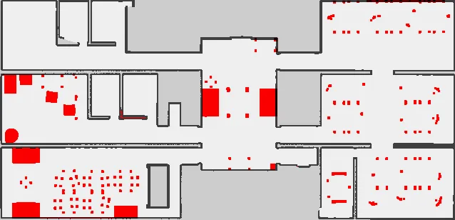
To explore the impact of unmapped obstacles in the environment, we decided to add an extra synthetic dataset. This dataset was generated in simulation, and consists of a differential robot navigating an office-like environment with frequent unmapped obstacles (desks, chairs, tables, and other furniture). Each bag file is about 30 minutes long. Figure 4 shows the map of the environment, and the location and relative size of the unmapped obstacles in it.

Results

The full output report generated by LAMBKIN for the benchmark can be found in this link.

For the time being, let’s focus our attention in the results for all datasets except the last. These are the same datasets used in a previous campaign: real-robot datasets and a simulated-robot 24hs long dataset, neither of which have unmapped obstacles in the environment.

We can see that for these datasets the likelihood_field_prob sensor model consistently outperforms the likelihood_field sensor model, with clearly separated confidence interval bands around the central values. The results are summarized in Figure 5.

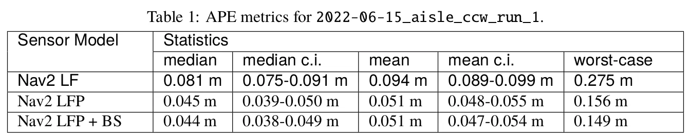
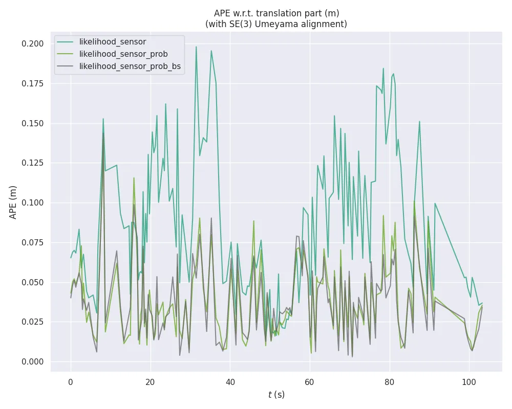
This difference in performance is visible also when looking at the evolution of the APE through time during the execution of a test: both likelihood_field_prob configurations tend to display lower values of APE than the likelihood_field sensor model. See Figure 6.

The beam skipping feature, however, does not seem to have a significant impact on the localization performance of the likelihood_field_prob sensor for most of the benchmarks.

But remember we said all of these datasets had no unmapped obstacles in them. What happens when we introduce unmapped obstacles in the environment?

Look both ways before crossing the street

Here’s where the additional dataset we included in this benchmarking campaign comes into play. This dataset is called “HQ Simulation” and the results for it can be found in the last chapter of the results report. Remember that this dataset consists of 30 minute-long bag files of a differential robot navigating an office-like environment with unmapped furniture.

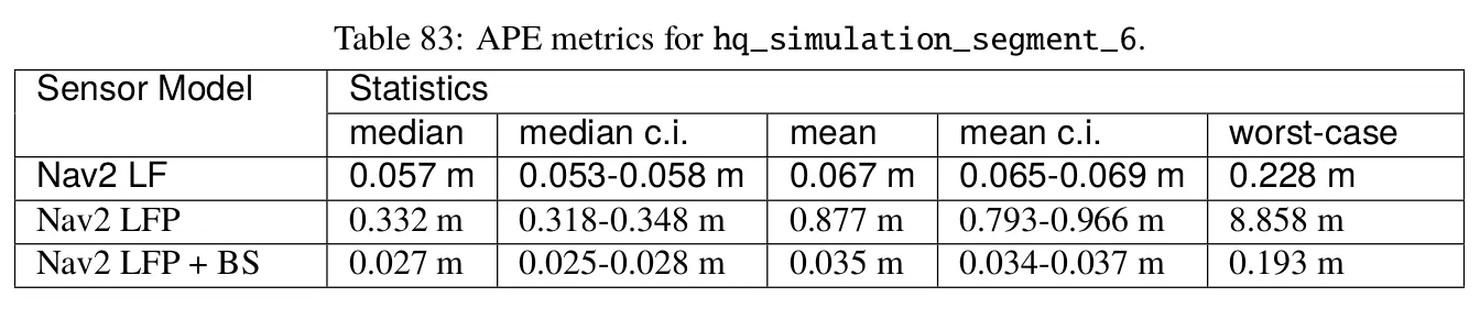
When looking at the results with this dataset we realized that the success story for likelihood_field_prob we saw before was not so clear-cut anymore, and that the sensor model was now performing noticeably worse than the regular likelihood_field sensor model for a significant number of bag files in this dataset. Interestingly, only the likelihood_field_prob sensor model with beam skipping disabled seemed to be having issues; whenever beam skipping was enabled, the performance would be consistent with that of the other datasets seen before. See for instance the results in Figure 7.

To determine why, we put these bag files under a magnifying glass. We looked into their logs, and we analyzed the localization performance in detail using evo. We also replayed them through RViz, to find out where in the map the pose tracking was lost, and whether the particle distribution and the estimated pose of the robot were affected by the environment right before these episodes.

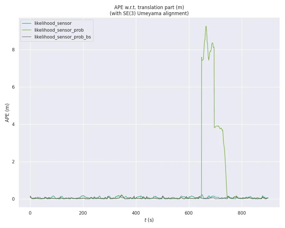
We found out that when the likelihood_field_prob sensor model is used with beam skipping disabled, the sensor model is prone to sudden divergences in the presence of unmapped obstacles, and that in practice this plays out as a very sudden change in the estimated pose. See for instance Figure 8, where around 640 seconds into the bag file the APE suddenly spikes up because the pose estimation was “instantaneously transported” to a different location in the map.

We also found out the reason to be of the beam skipping feature: When the likelihood_field_prob sensor model is used with beam skipping enabled, the sensor model is able to consistently track the true pose of the robot where the same filter with beam skipping disabled fails. Elsewhere, however, this feature does not seem to have any significant impact on the localization performance of the sensor model.

The difference in performance with the datasets discussed before seems to be because the product formula is very sensitive to unmapped obstacles: in their presence, a few of the beams in the scan will have very low likelihood values, and this will cause the weight of the particles to drop significantly. If enough beams are affected like this, the weights of the particles close to the true pose will become indistinguishable from the weights of any other particles that have partial matches with the environment. This can lead to unintentionally “selecting” an incorrect but numerically dominant hypothesis during the filter’s resampling step later.

The beam skipping feature seems to offer a protective mechanism against this weakness by filtering out beams that don’t fit the current hypothesis good enough, therefore avoiding low particle weights and random relocations of the tracked hypothesis.

Conclusion

From the data gathered we can see that there’s a lot of potential in the likelihood_field_prob sensor model, given that the localization performance of this sensor model is consistently better than the likelihood_field sensor model in all the datasets we evaluated.

Disabling the beam skipping feature is not recommended, however, since the sensor model is prone to sudden divergences in the presence of unmapped obstacles. Notice that beam skipping is disabled by default in the Nav2 AMCL, so this is something to keep in mind if you are using likelihood_field_prob in your robot.

The results of this benchmarking campaign are very promising, and they suggest that the likelihood_field_prob sensor model could be a good addition to the Beluga AMCL library, but further work is needed to improve its robustness, either with the inclusion of beam pre-filtering or some other mechanism.

Also, future work will try to evaluate the impact of the product formula for the beam model, to try to find out if similar performance improvements can be achieved.

Contact us

We hope you have found this article informative. If you have any questions or comments, feel free to reach out to us with your thoughts.

And if you happen to know the origin story of the nav2_amcl sum formula, we would love to hear it!